ATR or % Based Trailing Stop for Delta Exchange (trade_crush)This indicator calculates and visually displays a dynamic trailing stop line on the chart based on either the Average True Range (ATR) or a fixed percentage of the current close price. Designed especially for futures or crypto traders using Delta Exchange, it helps determine where to place trailing stop loss orders to manage risk effectively.
Cari dalam skrip untuk "Trailing stop"

Peter Brandt's 3-Day Trailing StopPeter Brandt's 3-day trailing stop rule is a trend-following exit strategy where a sell signal is triggered after a stock has reached a new high, followed by a close below the low of that high day, and then a break below the low of the next day, which is called the "setup day". The rule can be reversed to exit a short position. For long positions, Day 1 is the "high day" with a new price high, Day 2 is the "setup day" where the price closes below the low of Day 1, and Day 3 is the "trigger day" where a sell is executed if the price falls below the low of the setup day.
Long exit signal
Day 1: High Day: — The stock makes a new high.
Day 2: Setup Day: — The stock closes below the low of Day 1. At this point, the exit signal is now active.
Day 3: Trigger Day: — A sell to close is triggered when the price breaks below the low of the "setup day" (Day 2).
Short exit signal
Day 1: Low Day: — The stock makes a new low.
Day 2: Setup Day: — The stock closes above the high of Day 1.
Day 3: Trigger Day: — A buy to close is triggered when the price breaks above the high of the "setup day" (Day 2).

ATR Trailing Stop Without tradepanel Open✅ Only plots ATR trailing stop line
✅ Only colors candles
✅ No trades / entries
✅ No “Strategy Tester” panel
✅ No arrows, markers, or trade lists

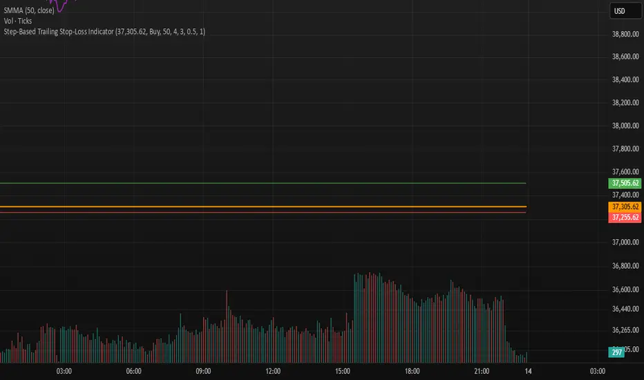
Step-Based Trailing Stop-Loss IndicatorThis indicator is built for momentum traders who want to maximize winning trades and minimize losses through a smart, step-based trailing stop-loss system. Instead of using a fixed Take Profit, this tool dynamically protects profits once the trade reaches a favorable RR (Risk-to-Reward) level.
How It Works:
Manual Entry Input
You enter your Entry Price and select Buy/Sell in the settings.
This flexibility allows backtesting or live trade tracking.
Initial Setup
Default SL: 50 ticks(Tested on us30,but works on any pair you just need to adjust SL)
TP for reference: 4R — can be used for benchmarking, but we don't limit profits with a hard TP.
Trailing Logic
Once price reaches 3R in profit:
The SL begins trailing.
It starts at 2R, keeping a 1R cushion behind the max profit.
For every 0.5R gain, SL also moves up by 0.5R:
Example: At 3.5R → SL is at 2.5R
At 5.0R → SL is at 4.0R
This trailing continues until the SL is hit or the trend exhausts.
Chart Features
🟧 Entry Line
🔴 Initial SL
🟢 Reference TP (4R, optional)
🟣 Dynamic Trailing SL
🏷️ Labels for Entry & SL levels
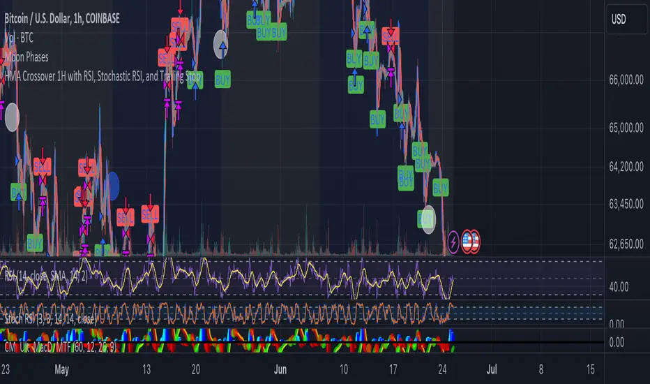
HMA Crossover 1H with RSI, Stochastic RSI, and Trailing StopThe strategy script provided is a trading algorithm designed to help traders make informed buy and sell decisions based on certain technical indicators. Here’s a breakdown of what each part of the script does and how the strategy works:
Key Components:
Hull Moving Averages (HMA):
HMA 5: This is a Hull Moving Average calculated over 5 periods. HMAs are used to smooth out price data and identify trends more quickly than traditional moving averages.
HMA 20: This is another HMA but calculated over 20 periods, providing a broader view of the trend.
Relative Strength Index (RSI):
RSI 14: This is a momentum oscillator that measures the speed and change of price movements over a 14-period timeframe. It helps identify overbought or oversold conditions in the market.
Stochastic RSI:
%K: This is the main line of the Stochastic RSI, which combines the RSI and the Stochastic Oscillator to provide a more sensitive measure of overbought and oversold conditions. It is smoothed with a 3-period simple moving average.
Trading Signals:
Buy Signal:
Generated when the 5-period HMA crosses above the 20-period HMA, indicating a potential upward trend.
Additionally, the RSI must be below 45, suggesting that the market is not overbought.
The Stochastic RSI %K must also be below 39, confirming the oversold condition.
Sell Signal:
Generated when the 5-period HMA crosses below the 20-period HMA, indicating a potential downward trend.
The RSI must be above 60, suggesting that the market is not oversold.
The Stochastic RSI %K must also be above 63, confirming the overbought condition.
Trailing Stop Loss:
This feature helps protect profits by automatically selling the position if the price moves against the trade by 5%.
For sell positions, an additional trailing stop of 100 points is included.
EMA and MACD with Trailing Stop Loss (by Coinrule)An exponential moving average ( EMA ) is a type of moving average (MA) that places a greater weight and significance on the most recent data points. The exponential moving average is also referred to as the exponentially weighted moving average. An exponentially weighted moving average reacts more significantly to recent price changes than a simple moving average simple moving average ( SMA ), which applies an equal weight to all observations in the period.
Moving average convergence divergence ( MACD ) is a trend-following momentum indicator that shows the relationship between two moving averages of a security’s price. The MACD is calculated by subtracting the 26-period exponential moving average ( EMA ) from the 12-period EMA.
The result of that calculation is the MACD line. A nine-day EMA of the MACD called the "signal line," is then plotted on top of the MACD line, which can function as a trigger for buy and sell signals. Traders may buy the security when the MACD crosses above its signal line and sell—or short—the security when the MACD crosses below the signal line. Moving average convergence divergence ( MACD ) indicators can be interpreted in several ways, but the more common methods are crossovers, divergences, and rapid rises/falls.
The Strategy enters and closes the trade when the following conditions are met:
LONG
The MACD histogram turns bearish
EMA7 is greater than EMA14
EXIT
Price increases 3% trailing
Price decreases 1% trailing
This strategy is back-tested from 1 January 2022 to simulate how the strategy would work in a bear market and provides good returns.
Pairs that produce very strong results include XRPUSDT on the 1-minute timeframe. This short timeframe means that this strategy opens and closes trades regularly
In order to further improve the strategy, the EMA can be changed from 7 and 14 to, say, EMA20 and EMA50. Furthermore, the trailing stop loss can also be changed to ideally suit the user to match their needs.
The strategy assumes each order is using 30% of the available coins to make the results more realistic and to simulate you only ran this strategy on 30% of your holdings. A trading fee of 0.1% is also taken into account and is aligned to the base fee applied on Binance.

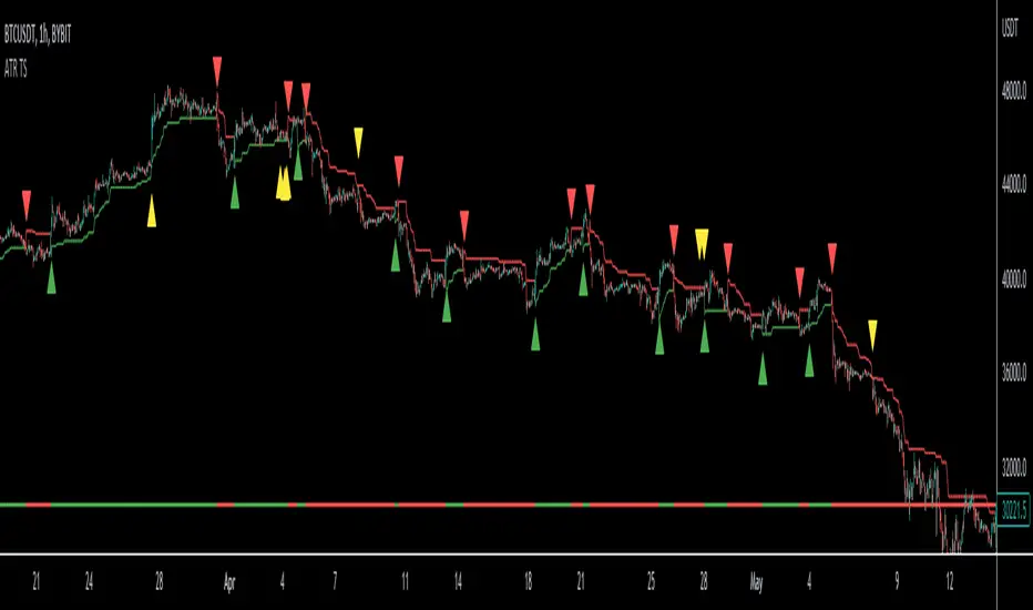
ATR Trailing Stop Loss [V5]A complete ATR Trailing Stop Loss in version 5.
Features Include:
Timeframe Option
Long/Short Triggers (Green/Red Triangles)
Long/Short Conditions (Bottom Colored Line)
"Golden" Long/Short Triggers (Yellow Triangles)(Hanging Man or Shooting Star Candlestick patterns breaking ATR trailing stop)
Alerts
PluePhantom's Trailing Stop Loss Multiple of ATRThis is a simple trailing stop loss line for long and short positions, made by Bluephantom using PS v2. I converted it onto v5
It is calculated as a multiple of the ATR instead of a percentage.
You are able to change the multiple and the ATR length.
It can be used as a guide to where you should consider putting in your stop loss on a trade and to where you should move your stop loss to as the days go by.
This indicator is experimental. Use at your own risk.

Rob Hoffman's 50/80/90/Price Trailing Stop LossA trailing stop loss method by Rob Hoffman.
Set your entry, TP, and SL.
Once price is 50% of its way to the TP, set your stop loss at the gray line.
Once price is 80% of its way to the TP, set your stop loss at the light gray line.
Once price is 90% of its way to the TP set your stop loss at the white line.

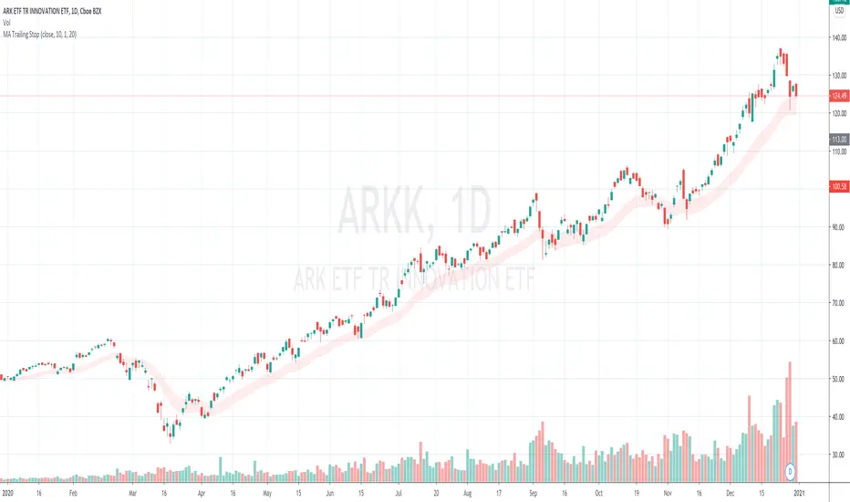
MA Trailing StopA Trailing Stop indicator that uses a multiple of ATR below a SMA/EMA line. Support long positions only.
Configurables:
1. Use SMA or EMA
2. MA Period
3. ATR multiplier
4. ATR look back period
The bottom of the red area indicates the stop line. The top of the red area indicates the reference MA line.
Ideal use case is you find your a red area that covers most local lows.
The stop line moves up with MA, but does not move down if MA moves down.
If moves down (re-calculates itself) only when a low penetrates the stop line.
Long Term Breakout entry + 25% Trailing stopThis script enters on a long term breakout and exits using a 25% trailing stop

Three Bar Exit Trailing Stop - Naked Forex: Price ActionThree Bar Exit Trailing Stop - Naked Forex: Exit indicator based on price action. The naked trader locks in profit by trailing the stop loss behind the lowest low of the last three candlesticks (for buy trades) or above the highest high of the last three candlesticks (For sell trades)

Simple Moving Average - ATR Trailing StopThe old adage goes "Cut losers fast and let the winners run"
With this in mind, this will plot a dynamic trailing stop by subtracting any multiplier of the Average True Range (ATR) from the SMA of your choice.

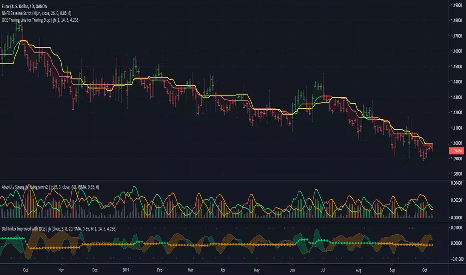
QQE Trailing Line for Trailing Stop | jhUsing parts of QQE (Qualitative Quantitative Estimation) again, this time I'm applying the trailing line of QQE on price directly.
Outcome, it's behaving like a baseline filter and it can be use as an exit or a trailing stop indicator.
As comparing to Kijun-sen line in yellow, the QQE trailing line follows the price closer, therefore exiting you sooner when the trend direction changes.
There's 2 QQE option, they behave differently during the trend change.
Credits to Glaz and Shizaru for their QQE code.
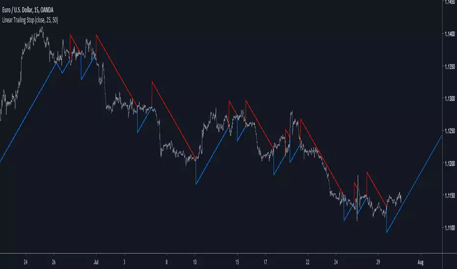
Linear Trailing StopBased on my latest script "Linear Channels"
This is a trailing stop version of the linear channels. Thanks to capissimo for helping me fix several issues with the linear extrapolation part.
In order to know how the indicator work i recommend reading the post on the Linear Channels indicator here
Hope you like it and feel free to leave your suggestions :)
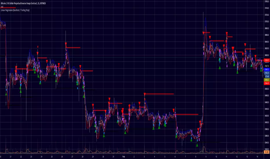
Linear Regression (Backtest / Trailing Stop)A Strategy with Backtest and Trailing Stop for Long/Short
Credits: Study by RafaelZioni - Thanks buddy!
ATR Trailing Stop Bands Strategy [R] Originally based on a script by HPotter for an ATR Trailing Stop, which itself was based on an article by Sylvain Vervoort, but I adapted it to add Bands, to add extra optional Wick Protection, and have now made it a Strategy. It's not great for entries/exits, but as a Trailing Stop that can let winners ride, it's great.

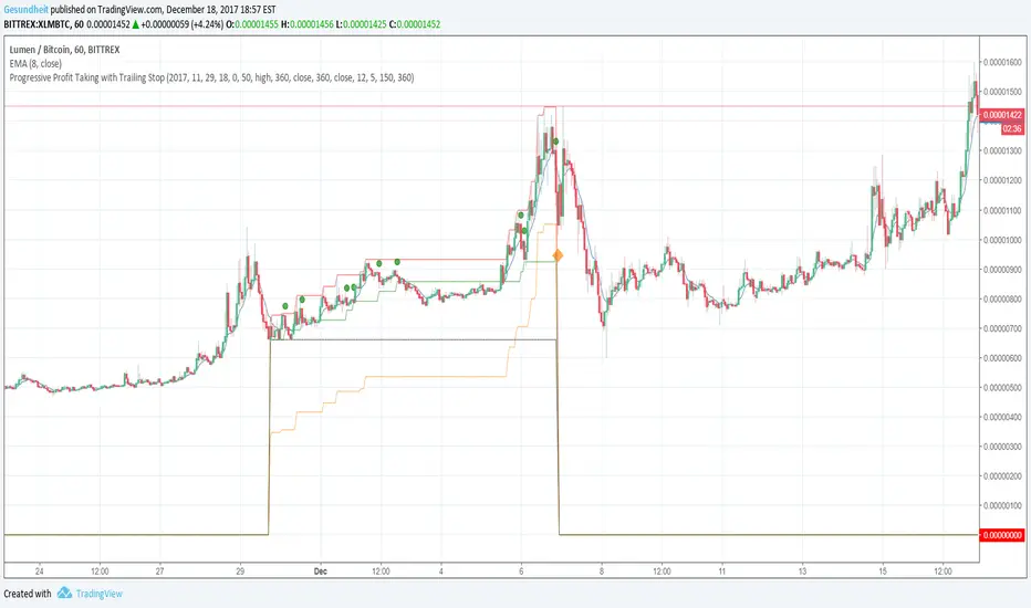
Progressive Profit Taking with Trailing StopThis is version 2 of
Special features:
Added partial profit taking as price rises. Profit taking is triggered by price crossing an EMA.
After profit taking, price has to rise by a user-specified percent before taking profits again.
Also includes condition for fully closing position after meeting specified profit target.
To incorporate into your algo, turn the plotshape functions into alertcondition.
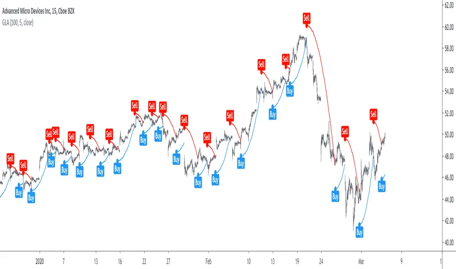
Grover Llorens Activator [alexgrover & Lucía Llorens] Trailing stops play a key role in technical analysis and are extremely popular trend following indicators. Their main strength lie in their ability to minimize whipsaws while conserving a decent reactivity, the most popular ones include the Supertrend, Parabolic SAR and Gann Hilo activator. However, and like many indicators, most trailing stops assume an infinitely long trend, which penalize their ability to provide early exit points, this isn't the case of the parabolic SAR who take this into account and thus converge toward the price at an increasing speed the longer a trend last.
Today a similar indicator is proposed. From an original idea of alexgrover & Lucía Llorens who wanted to revisit the classic parabolic SAR indicator, the Llorens activator aim to converge toward the price the longer a trend persist, thus allowing for potential early and accurate exit points. The code make use of the idea behind the price curve channel that you can find here :
I tried to make the code as concise as possible.
The Indicator
The indicator posses 2 user settings, length and mult , length control the rate of convergence of the indicator, with higher values of length making the indicator output converge more slowly toward the price. Mult is also related with the rate of convergence, basically once the price cross the trailing stop its value will become equal to the previous trailing stop value plus/minus mult*atr depending on the previous trailing stop value, therefore higher values of mult will require more time for the trailing stop to reach the closing price, use higher values of mult if you want to avoid potential whipsaws.
Above the indicator with slow convergence time (high length) and low mult.
Points with early exit points are highlighted.
Usage For Oscillators
The difference between the closing price and an overlay indicator can provide an oscillator with characteristics depending on the indicators used for differencing, Lucía Llorens stated that we should find indicators for differencing that highlight the cycles in the price, in other terms : Price - Signal , where we want to find Signal such that we maximize the visibility of the cycles, it can be demonstrated that in the case where the closing price is an additive model : Trend + Cycles + Noise , the zero lag estimation of the Trend component can allow for the conservation of the cycle and noise component, that is : Price - Estimate(Trend) , for example the difference between the price and moving average isn't optimal because of the moving average lag, instead the use of zero lag moving averages is more suitable, however the proposed indicator allow for a surprisingly good representation of the cycles when using differencing.
The normalization of this oscillator (via the RSI) allow to make the peak amplitude of the cycles more constant. Note however that such method can return an output with a sign inverse to the one of the original cycle component.
Conclusion
We proposed an indicator which share the logic of the SAR indicator, that is using convergence toward the price in order to provide early exit points detection. We have seen that this indicator can be used to highlight cycles when used for differencing and i don't exclude publishing more indicators based on this method.
Lucía Llorens has been a great person to work with, and provided enormous feedback and support while i was coding the indicator, this is why i include her in the indicator name as well as copyright notice. I hope we can make more indicators togethers in the future.
(altho i was against using buy/sells labels xD !)
Thanks for reading !
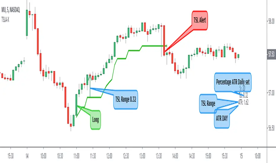
Trailing Stop Loss ATR + AlertI share this TSL indicator with alert (I use it only for Stocks), the configuration is very simple, you must select if it is a Short or Long operation, time at which the operation was opened,% of the daily ATR for TSL. It also contains:
- Alert
- Panel Info
Trailing Stop LossThis script demonstrate how to make a Training Stop Loss to "ride the wave". In comparison to classic Stop Loss this strategy follows the price upwards (for long positions) and when price drops by a fixed percentage then you exit your position.

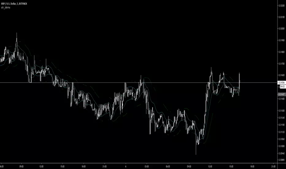
atr_idemaTrailing stop indicator.
Trail when the top/bottom green line appears (with that line value as stop price).